Semantic Image Segmentation using FCNs

What is it about?

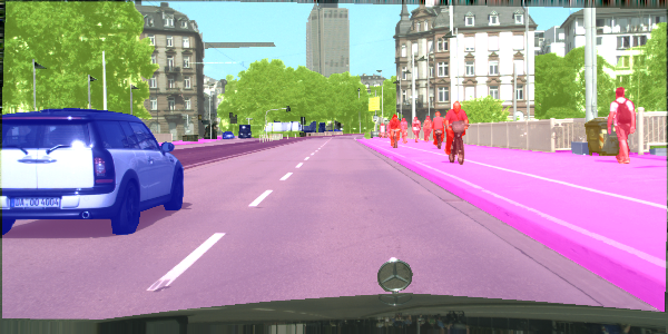
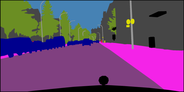
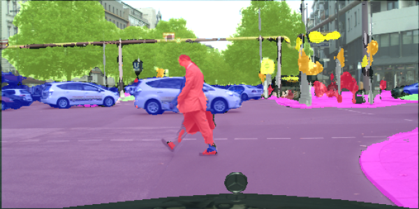
Semantic segmentation is a process of dividing an image into sets of pixels sharing similar properties and assigning to each of these sets one of the pre-defined labels. Ideally, you would like to get a picture such as the one below. It's a result of blending color-coded class labels with the original image. This sample comes from the CityScapes dataset.

Segmented Image

Segmentation Classes

How is it done?

Figuring out object boundaries in an image is hard. There's a variety of "classical" approaches taking into account colors and gradients that obtained encouraging results, see this paper by Shi and Malik for example. However, in 2015 and 2016, Long, Shelhamer, and Darrell presented a method using Fully Convolutional Networks that significantly improved the accuracy (the mean intersection over union metric) and the inference speed. My goal was to replicate their architecture and use it to segment road scenes.

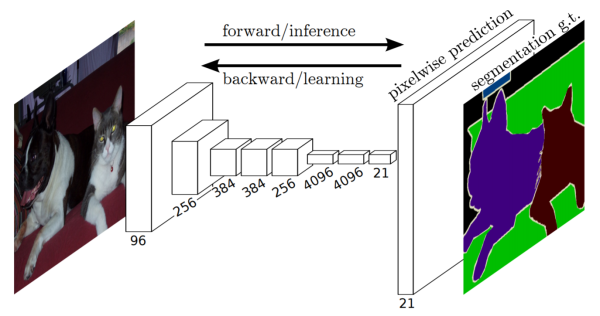
A fully convolutional network differs from a regular convolutional network in the fact that it has the final fully-connected classifier stripped off. Its goal is to take an image as an input and produce an equally-sized output in which each pixel is represented by a softmax distribution describing the probability of this pixel belonging to a given class. I took this picture from one of the papers mentioned above:

Fully Convolutional Network

For the results presented in this post, I used the pre-trained VGG16 network provided by Udacity for the beta test of their Advanced Deep Learning Capstone. I took layers 3, 4, and 7 and combined them in the manner described in the picture below, which, again, is taken from one of the papers by Long et al.

Upscaling and merging

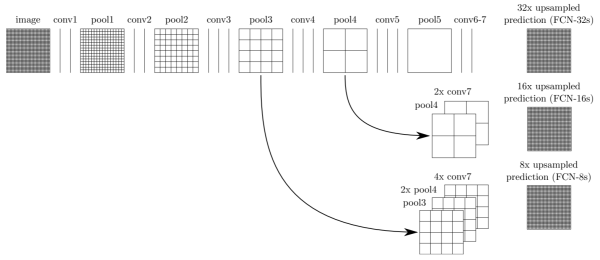
First, I used a 1x1 convolutions on top of each extracted layer to act as a local classifier. After doing that, these partial results are still 32, 16, and 8 times smaller than the input image, so I needed to upsample them (see below). Finally, I used a weighted addition to obtain the result. The authors of the original paper report that without weighting the learning process diverges.

Learnable Upsampling

Upsampling is done by applying a process called transposed convolution. I will not describe it here because this post over at cv-tricks.com does a great job of doing that. I will just say that transposed convolutions (just like the regular ones) use learnable weights to produce output. The trick here is the initialization of those weights. You don't use the truncated normal distribution, but you initialize the weights in such a way that the convolution operation performs a bilinear interpolation. It's easy and interesting to test whether the implementation works correctly. When fed an image, it should produce the same image but n times larger.

 1img = cv2.imread(sys.argv[1])
 2print('Original size:', img.shape)
 3
 4imgs = np.zeros([1, *img.shape], dtype=np.float32)
 5imgs[0,:,:,:] = img
 6
 7img_input = tf.placeholder(tf.float32, [None, *img.shape])
 8upscale = upsample(img_input, 3, 8, 'upscaled')
 9
10with tf.Session() as sess:
11    sess.run(tf.global_variables_initializer())
12    upscaled = sess.run(upscale, feed_dict={img_input: imgs})
13
14print('Upscaled:', upscaled.shape[1:])
15cv2.imwrite(sys.argv[2], upscaled[0,:, :, :])

Where upsample is defined here.

Datasets

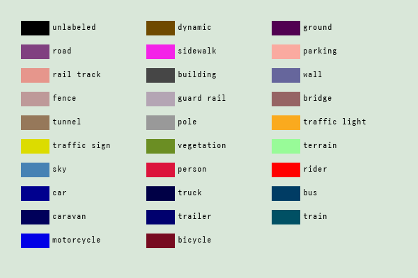
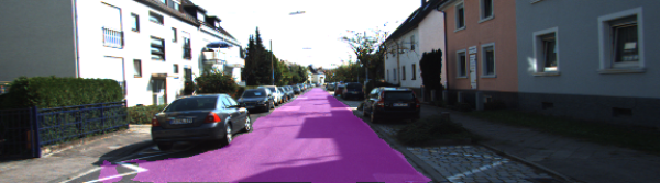
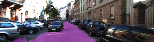
I was mainly interested in road scenes, so I played with the KITTI Road and CityScapes datasets. The first one has 289 training images with two labels (road/not road) and 290 testing samples. The second one has 2975 training, 500 validation, and 1525 testing pictures taken while driving around large German cities. It has fine-grained annotations for 29 classes (including "unlabeled" and "dynamic"). The annotations are color-based and look like the picture below.

Picture Labels

Even though I concentrated on those two datasets, both the training and the inference software is generic and can handle any pixel-labeled dataset. All you need to do is to create a new source_xxxxxx.py file defining your custom samples. The definition is a class that contains seven attributes:

image_size - self-evident, both horizontal and vertical dimensions need to be divisible by 32
num_classes - number of classes that the model is supposed to handle
label_colors - a dictionary mapping a class number to a color; used for blending of the classification results with input image
num_training - number of training samples
num_validation - number of validation samples
train_generator - a generator producing training batches
valid_generator - a generator producing validation batches

See source_kitti.py or source_cityscapes.py for a concrete example. The training script picks the source based on the value of the --data-source parameter.

Normalization

Typically, you would normalize the input dataset such that its mean is at zero and its standard deviation is at one. It significantly improves convergence of the gradient optimization. In the case of the VGG model, the authors just zeroed the mean without scaling the variance (see section 2.1 of the paper). Assuming that the model was trained on the ImageNet dataset, the mean values for each channel are muR = 123.68, muG = 116.779, muB = 103.939. The pre-trained model provided by Udacity already has a pre-processing layer handling these constants. Judging from the way it does it, it expects plain BGR scaled between 0 and 255 as input.

Label Validation

Since the network outputs softmaxed logits for each pixel, the training labels need to be one-hot encoded. According to the TensorFlow documentation, each row of labels needs to be a proper probability distribution. Otherwise, the gradient calculation will be incorrect and the whole model will diverge. So, you need to make sure that you're never in a situation where you have all zeros or multiple ones in your label vector. I have made this mistake so many time that I decided to write a checker script for my data source modules. It produces examples of training images blended with their pixel labels to check if the color maps have been defined correctly. It also checks every pixel in every sample to see if the label rows are indeed valid. See here for the source.

Initialization of variables

Initialization of variables is a bit of a pain in TensorFlow. You can use the global initializer if you create and train your model from scratch. However, in the case when you want to do transfer learning - load a pre-trained model and extend it - there seems to be no convenient way to initialize only the variables that you created. I ended up doing acrobatics like this:

1uninit_vars    = []
2uninit_tensors = []
3for var in tf.global_variables():
4    uninit_vars.append(var)
5    uninit_tensors.append(tf.is_variable_initialized(var))
6uninit_bools = sess.run(uninit_tensors)
7uninit = zip(uninit_bools, uninit_vars)
8uninit = [var for init, var in uninit if not init]
9sess.run(tf.variables_initializer(uninit))

Training

For training purposes, I reshaped both labels and logits in such a way that I ended up with 2D tensors for both. I then used tf.nn.softmax_cross_entropy_with_logits as a measure of loss and used AdamOptimizer with a learning rate of 0.0001 to minimize it. The model trained on the KITTI dataset for 500 epochs - 14 seconds per epoch on my GeForce GTX 1080 Ti. 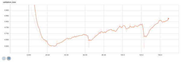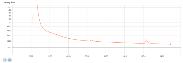The CityScapes dataset took 150 epochs to train - 9.5 minutes per epoch on my GeForce vs. 25 minutes per epoch on an AWS P2 instance. 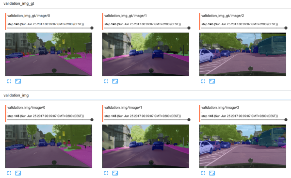The model exhibited some overfitting. However, the visual results seemed tighter the more it trained. In the picture below the top row contains the ground truth, the bottom one contains the inference results (TensorBoard rocks! :).

CityScapes Validation Examples

CityScapes Validation Loss

CityScapes Training Loss

Results

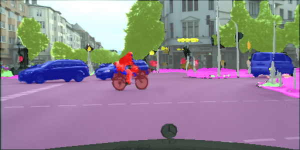
The inference (including image processing) takes 80 milliseconds per image on average for CityScapes and 27 milliseconds for KITTI. Here are some examples from both datasets. The model seems to be able to distinguish a pedestrian from a bike rider with some degree of accuracy, which is pretty impressive!