Intro
I have recently spent a non-trivial amount of time building an SSD detector from scratch in TensorFlow. I had initially intended for it to help identify traffic lights in my team's SDCND Capstone Project. However, it turned out that it's not particularly efficient with tiny objects, so I ended up using the TensorFlow Object Detection API for that purpose instead. In the end, I managed to bring my implementation of SSD to a pretty decent state, and this post gathers my thoughts on the matter. It is not intended to be a tutorial. Instead, it's a discussion of all the pieces of information that were unclear to me or that I needed to research independently of the original paper.
Base Network and Extensions
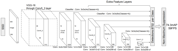
SSD is based on a modified VGG-16 network pre-trained on the ImageNet data. I happened to have one from one of my previous projects, and I used it here as well. The following modifications have been made to the base network:
pool5was changed from 2x2 (stride: 2) to 3x3 (stride: 1)fc6andfc7were converted to convolutional layers and subsampled- à trous convolution was used in
fc6 fc8and all of the dropout layers were removed
As you can see from the above image, the fc6 and fc7 convolutions are
3x3x1024 and 1x1x1024 respectively, whereas in the original VGG they are
7x7x4096 and 1x1x4096. Having huge filters like these is a computational
bottleneck. According to one of the references, we can address this
problem by "spatially subsampling (by simple decimation)" the weights and then
using the à trous convolution to keep the filter's receptive field unchanged.
It was not immediately clear to me what it means, but after reading
this page of MatLab's documentation, I came up the following:
with tf.variable_scope('mod_conv6'):
    orig_w, orig_b = sess.run([self.vgg_fc6_w, self.vgg_fc6_b])
    mod_w = np.zeros((3, 3, 512, 1024))
    mod_b = np.zeros(1024)

    for i in range(1024):
        mod_b[i] = orig_b[4*i]
        for h in range(3):
            for w in range(3):
                mod_w[h, w, :, i] = orig_w[3*h, 3*w, :, 4*i]

    w = array2tensor(mod_w, 'weights')
    b = array2tensor(mod_b, 'biases')
    x = tf.nn.atrous_conv2d(self.mod_pool5, w, rate=6, padding='SAME')
    x = tf.nn.bias_add(x, b)
    self.mod_conv6 = tf.nn.relu(x)
It doubled the speed of training and did not seem to have any adverse effects on accuracy. Note that the dilation rate of the à trous convolution is set to 6 instead of 3. This setting is inconsistent with the size of the original filter, but it is nonetheless used in the reference code.
The output of the conv4_3 layer differs in magnitude compared to other layers
used as feature maps of the detector. As pointed out in the ParseNet
paper, this fact may lead to reduced performance because "larger" features may
overwhelm the "smaller" ones. They propose to use L2 normalization with a scale
learnable separately for each channel as a remedy to this problem. This is what
I ended up doing in TensorFlow:
def l2_normalization(x, initial_scale, channels, name):
    with tf.variable_scope(name):
        scale = array2tensor(initial_scale*np.ones(channels), 'scale')
        x = scale*tf.nn.l2_normalize(x, dim=-1)
    return x
The initial scale for each channel is set to 20, and it does not change very much over the training time.
Furthermore, a bunch of extra convolutional layers were added on top of the
modified fc7. The number of these layers depends on the flavor of the
detector: vgg300 or vgg512. The paper does not explain well enough the
parameters of the convolutions, especially the padding settings, even though
getting this part wrong can significantly impact the performance. I looked these
up in the reference code for vgg300 and worked my way backward from
the number of anchors in the case of vgg512. Here's what I ended up with:
conv8_1: 1x1x256 (stride: 1, pad: same)conv8_2: 3x3x512 (stride: 2, pad: same)conv9_1: 1x1x128 (stride: 1, pad: same)conv9_2: 3x3x256 (stride: 2, pad: same)conv10_1: 1x1x128 (stride: 1, pad: same)conv10_2: 3x3x256 (stride: 1, pad: valid) forvgg300, (stride: 2, pad: same) forvgg515conv11_1: 1x1x128 (stride: 1, pad: same)conv11_2: 3x3x256 (stride: 1, pad: valid)
For the vgg512 flavor, there are two extra layers:
conv12_1: 1x1x128 (stride: 1, pad: same)- padding of the
conv12_1feature map with one extra cell in each spacial dimension conv12_2: 3x3x256 (stride: 1, pad: valid)
It's not possible to use the predefined padding options (VALID or SAME) for extending
conv12_1, so I ended doing it manually:
x, l2 = conv_map(self.ssd_conv11_2, 128, 1, 1, 'conv12_1')
paddings = [[0, 0], [0, 1], [0, 1], [0, 0]]
x = tf.pad(x, paddings, "CONSTANT")
self.ssd_conv12_1 = self.__with_loss(x, l2)
x, l2 = conv_map(self.ssd_conv12_1, 256, 3, 1, 'conv12_2', 'VALID')
self.ssd_conv12_2 = self.__with_loss(x, l2)
Default Boxes (a. k. a. Anchors)
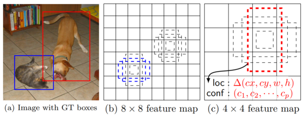
The model takes the outputs of some of these convolutional layers and associates a scale with each of them. The exact formula is presented in the paper; the reference implementation does not seem to follow it exactly, though. In general, the further away the feature map is from the input, the larger is the scale assigned to it. The scale only loosely correlates with the receptive field of the respective filter.
The model adds a bunch of 3x3xp convolutional filters on top of each of these maps. Each of these filters predicts p parameters of a default box (or an anchor) at the location to which it is applied. Four of these p parameters are the coordinates of the window (relative width and height, as well as x and y offsets from the center of the anchor). The remaining parameters define the probability distribution of the box belonging to one of the classes that the model predicts (the softmaxed logits). We need to add as many of these filters per feature map as we want aspect ratios for the default boxes of a given scale. In general, the more, the better. The paper advises using six aspect ratios per map. However, the implementation uses fewer of them in some cases.
We now need to create the ground truth labels for the optimizer. We match each ground truth box to an anchor box with the highest Jaccard overlap (if it exceeds 0.5). Additionally, we match it to every anchor with overlap higher than 0.5. The original code uses a mixture of bipartite matching and maximum overlap to resolve conflicts, but I just used the latter criterion for simplicity. For every matched anchor we set the class label accordingly and use the following for the box parameters:
\[ w = 10 \cdot log(\frac{w_{gt}}{w_{a}}) \\ h = 10 \cdot log(\frac{h_{gt}}{h_{a}}) \\ x_c = 5 \cdot \frac{x_{c,gt} - x_{c,a}}{w_a} \\ y_c = 5 \cdot \frac{y_{x,gt} - y_{c,a}}{h_a} \]The code uses the scaling constants above (5, 10) and calls them "prior variance," but the paper does not mention this fact.
Training Objective
The loss function consists of three parts:
- the confidence loss
- the localization loss
- the l2 loss (weight decay in the Caffe parlance)
The confidence loss is what TensorFlow calls softmax_cross_entropy_with_logits,
and it's computed for the class probability part of the parameters of each
anchor. Since there are many more positive (matched) anchors than negative
(unmatches/background) ones, the learning ends up being more stable if not every
background score contributes to the final loss. We need to mine the scores of all
the positive anchors and at most three times as of many negative anchors. We only
use the background anchors with the highest confidence loss. It results in
a somewhat involved code in the declarative style of TensorFlow.
The localization loss sums up the Smooth L1 losses of differences between the prediction and the ground truth labels. The Smooth L1 loss is defined as follows:
\[ SmoothL1(x) = \begin{cases} |x| - 0.5 & x \geq 1 \\ 0.5 \cdot x^2 & x \lt 1 \\ \end{cases} \]It translates to the following code in TensorFlow:
def smooth_l1_loss(x):
    square_loss   = 0.5*x**2
    absolute_loss = tf.abs(x)
    return tf.where(tf.less(absolute_loss, 1.), square_loss, absolute_loss-0.5)
The paper advises using the batch size of 32. However, this recommendation
assumes training in parallel on four GPUs. If you have just one (like I do), 8
is a better number. The original code uses the SGD optimizer with momentum,
rate decay at predefined steps, and doubling of the rate for biases. I found
that using the Adam optimizer with the exponential decay rate of 0.97 per epoch
and using 0.1 as the stability constant (epsilon) works better for this
implementation. The TensorFlow documentation warns that the default epsilon
may not be a good choice in general and recommends using a higher value in some
cases. Indeed, I found that using the default makes the weights very small very
fast and the learning process becomes unstable.
Non-Maximum Suppression
Because of the anchor matching strategy and the vast irregularity of the shapes we train on, the network will produce multiple overlapping detections of the same object. One way to get rid of duplicates is to perform a non-maxima suppression. The algorithm is straightforward:
- you pick your favorite box
- you remove all the boxes that have the Jaccard overlap with your selection above a certain threshold
- you choose your second favorite box and repeat step 2
- you continue until there is no new favorite to select
This article provides a more detailed description, although their selection criterion is rather strange (the position of the lower-right corner) and the implementation is pretty inefficient. My code using numpy's bulk operations is here. I should reimplement it using TensorFlow tensors and will likely do that when I have a spare moment.
Data Augmentation and Issues with Parallelism in Python
The SSD training depends heavily on data augmentation. I won't describe it at all here because the paper does a great job at that. The only tricky part that it does not mention is the fact that you do not clip any ground truth box if it happens to span outside the boundaries of a subsampled input image. See transforms.py if you want more details.
Things run much faster when the data is preprocessed in parallel before being fed to TensorFlow. However, the poor support for multithreading/multiprocessing in Python turned out to be a significant obstacle here. As you probably know, running your computation in multiple threads is utterly pointless in Python because the execution ends up being serial due to GIL issues. The GIL problem is typically addressed with multiprocessing. However, it comes with a separate can of worms.
First, if you want to transfer any significant amount of data between the processes efficiently, you need to avoid pickling and use the POSIX shared memory instead. It's not hugely complicated, but it's not trivial either. Second, if any of the packages you import uses threading underneath, you're almost guaranteed to encounter fork-safety issues. Add strange errors while forking CUDA-enabled libraries to the mix and you end up with a minor horror story. It took me about a full day of work to write and debug the shared memory queue and to debug the fork safety issues in the pipeline. In case you wonder, this code does the trick for the latter:
workers = []
os.environ['CUDA_VISIBLE_DEVICES'] = ""
cv2_num_threads = cv2.getNumThreads()
cv2.setNumThreads(1)
for i in range(num_workers):
    args = (sample_queue, batch_queue)
    w = mp.Process(target=batch_producer, args=args)
    workers.append(w)
    w.start()
del os.environ['CUDA_VISIBLE_DEVICES']
cv2.setNumThreads(cv2_num_threads)
Pascal VOC and the mAP Metric
The Pascal VOC (Visual Object Classes) project provides standardized datasets for object class recognition as well as tools for evaluation and comparison of different detection methods. The datasets contain several thousands of annotated Flickr pictures. The metric they use for method comparison of object detection algorithms is called mAP - Mean Average Precision - and is an arithmetic mean of the AP (Average Precision) scores for each object class in the dataset.
The task of object detection is treated as a ranked document retrieval system (as in search) and the AP metric is an 11-point interpolated average precision. More specifically, the system:
- sorts the detections of a given class in all the images of the dataset by confidence in descending order
- loops over the detections and classifies them according to the following
greedy algorithm:
- if a detection overlaps with the ground truth object with the IoU score of 50% or more and the object has not been previously detected, it's a true positive
- if IoU is above 50% but the object has been detected before, or the IoU is below 50%, it's a false positive
- ground truth object with no matching detections are false negatives
- calculate the precision and recall for the current state
Precision and recall data points calculated at each iteration contribute to the precision vs. recall curve which is then interpolated according to the following formula, sampled at 11 equally spaced recall points between 0 and 1, and averaged.
\[ p_{interp}(r) = \max_{r' \geq r} p(r') \]The graph below shows what the curves for the bottle class look like when we decide to accept objects above different confidence thresholds. Note how the curves for lower confidence levels extend the ones for the higher levels.
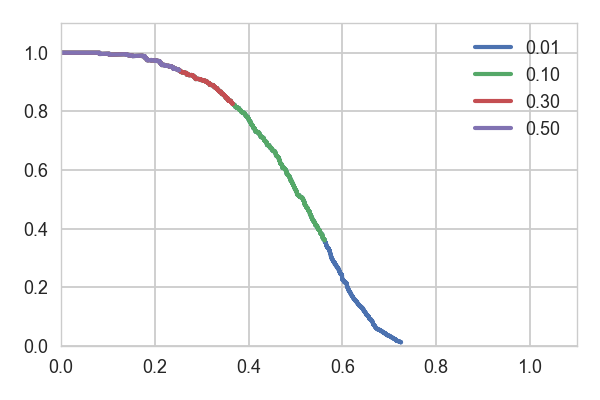
Here are the AP values for the corresponding confidence thresholds:
| Confidence | AP |
|---|---|
| 0.01 | 0.497 |
| 0.10 | 0.471 |
| 0.30 | 0.353 |
| 0.50 | 0.270 |
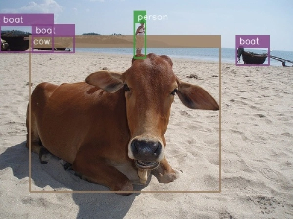
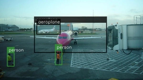
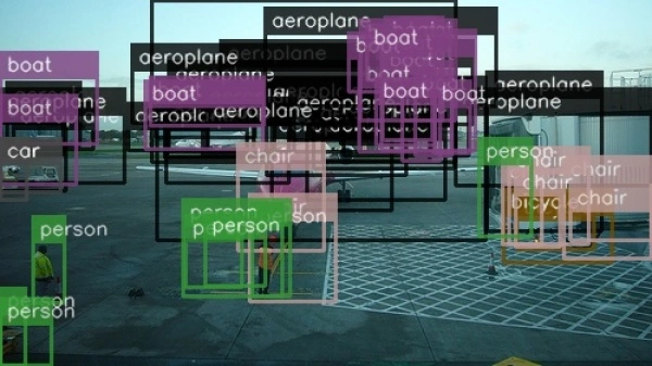
The lower confidence results we're willing to accept, the higher our AP gets, but also the number of low confidence false positives grows. It makes perfect sense for a ranked document retrieval system. We care a lot whether we get only the relevant results in the first couple of pages of a Google search, but we don't care all that much if we have a bunch of false positives on the hundredth page. Does it make sense when it comes to object detection? That probably varies widely depending on your application. I would argue that, in a general case, when you just care about quality detections, it's somewhat confusing. Below are examples of detections in the same picture with boxes above 0.5 and 0.01 confidence levels coming from the same SSD model. The parameters used to produce the second picture score higher mAP over the entire dataset than the ones used to generate the first one.
You can get more info about it here.
Results
I trained a somewhat modified version of the vgg300 flavor of the detector on
the union of VOC2007+VOC2012 trainval and VOC2007 test samples with heavy data
augmentation. It scored 74.7% mAP when tested on the samples it trained on, while
the reference score is around 77.5%. The result on the VOC2012 test samples was
68.71% with the reference at 75.8%. I did not use the same aspect
ratio and scale settings as the ones utilized by the original implementation.
Surprisingly, sticking to the reference parameters produced even worse results.
Another reason for the discrepancy may be a different choice of the optimizer
and the fact that the reference implementation doubles the learning rate for
biases. Using different learning rates for different variables is possible
in TensorFlow. However, I have not been able to do that without the system
repeating the forward pass and most of the backward pass for each learning rate
setting. It effectively almost doubled the training time per epoch, and I was not
patient enough to wait for the results.
When I exported the model as a static inference graph, it took roughly 100MB, compared to around 1.3GB when in the checkpoint format. I then used it as a detector in the vehicle detection project I did some time ago. It processed 1261 frames of the testing video, including the FFmpeg compression and decompression time, in roughly 25 seconds reaching over 50 FPS on average. It's a blazing speed considering that my fairly inefficient SVM implementation took well over 8 minutes (~2.5 FPS) to process the same video. Note, however, that, due to the non-maximum suppression, the speed is a function of the number of positive predictions, and this video has relatively few detected objects. You can see the results below.
Conclusion
The project took quite a bit longer than I had initially anticipated but it
was a great learning experience and ultimately a great deal of fun. With the
hard negative mining, it was probably the most complicated loss function I have
implemented in TensorFlow to date. I learned about adaptive feature map scaling,
dug through a lot of Caffe's and TensorFlow's source code, learned about the
stability of AdamOptimizer, and read a whole bunch of deep learning research
papers. I wasted some time fighting mostly non-existent issues because I had not
initially paid sufficient attention to what is measured by the accuracy metric.
I have a bunch of ideas on how to improve the model to reach the reference
performance and I will likely try some of them out in the near future.
All my code is here.
Update 10.03.2018: I have had a look at the PyTorch SSD implementation which achieves better results than mine in the VOC2012 test, but still lower than the baseline. I discovered that the way I did the data augmentation reflected what the paper describes but not what the original Caffe implementation does. I have updated the code in the repo to match the reference. I have also discovered a bug where the ground truth boxes produced by the sampler were sometimes too small to match any anchors. This behavior did not cause any runtime errors, but such samples did not contribute to the loss function and, therefore, had no impact on the optimization process. With these two changes, I was able to shrink the number of anchors used by my models to the level of the original implementation and reproduce my previous results. The performance of my code is still somewhat behind the original one. At this point, I am reasonably sure it's because of the base network weights I used. I will have a look at that when I have a spare moment.
Update 16.08.2020: I have just noticed that the post has not been updated to reflect the fact that my implementation does reproduce the performance results of the original paper after some more tweaks. Please see the GitHub repo for details.